Apache Spark is a distributed computing engine designed for fast and large-scale data processing. it can handle both batch and real-time streaming data, and it offers built-in libraries for machine learning, graph analytics, and SQL-like querying. At its core, Spark introduces the idea of in-memory computation. instead of writing intermediate results back to disk (like hadoop's mapreduce), spark stores them in memory whenever possible, drastically speeding up computations Spark supports multiple data abstractions:

• RDD (Resilient Distributed Dataset): the fundamental building block– a fault-tolerant collection of data distributed across a cluster
• DataFrame: a higher-level API built on RDDs, optimized and similar to SQL tables
• Dataset (Scala/Java only): type-safe version of dataframe

Why?

Before spark, hadoop mapreduce was the go-to tool for large-scale data processing. However:

1. Slow Iterative Processing: Each MapReduce stage required disk reads/writes
2. Limited APIs: Writing MapReduce jobs in Java was verbose and hard to debug
3. Lack of unification: batch jobs, streaming and ML required different tools Spark solves these issues:

• Speed: up to 100x faster than MapReduce (thanks to in-memory execution)
• Ease of Use: APIs in Python, Scala, Java, R
• Scalability: runs on laptops, clusters or in the cloud Applied to recommendation systems: Recommendation algorithms often require iterative matrix factorizations, graph traversals, and aggregations across billions of user-item interactions, Spark makes these feasible by distributing work across many nodes.

When?

• Big Data Scenarios: data too large to fit on a single machine
• Iterative ML Algorithms: e.g., collaborative filtering, gradient descent
• Data pipelines: ETL (extract, transform, load) on massive logs
• Real-Time Analysis: Monitoring user activity streams

How?

1. Driver program: coordinates the overall job
2. Cluster manager (standalone, YARN, Mesos, Kubernetes): allocates resources
3. Executors: Run computation on worker nodes
4. Tasks: Small units of work executed by executors Data flows through two key steps:

• Transformations (lazy ) -> Define operations (map, filter, join)
• Actions (trigger execution) -Z force computation (count, collect, save)

# Load dataset
data = spark.read.csv("/data/interactions.csv", headers=True)

# Transformations: Filter ratings >= 4
postive = data.fitler(data["rating"] >= 4)

# Action: Count rows
positive.count()

in this example

• filter() is a transformation
• count() is an action

Basics and Transformations

Transformations in spark are operations that define a new dataset from an existing one, they are lazy: Spark does not execute them immediately, it just builds a lineage (DAG, direcated acyclic graph) of steps, the actual computation happens only when an action (line count(), collect() or save()) is called the design has two major advantages:

1. Optimization: spark can analyze the entire workflow and reorganize it for efficiency
2. Fault tolerance: if part of the data is lost, Spark can recompute it using the lineage

Types of Transformations

Transformations are broadly divided into two categories:

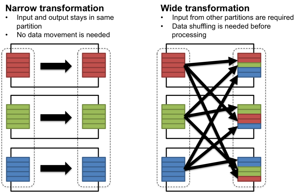
1. Narrow transformations

• Data required to compute the output comes from a single partition of the parent RDD/Dataframe
• No shuffling between nodes
• Examples:
  • map(): apply a function to each record
  • filter(): keep only records matching a condition
  • flatMap(): like map(), but output can expand into multiple records Applied example(recsys context): filter ratings ≥ 4 before training a model

ratings = spark.read.csv("ratings.csv", headers=True, inferSchema=True)
positive_ratings = ratings.filter(ratings["ratings"] >= 4)

here, each partition is filtered independently, no data movement required

2. Wide transformations

• Output requires data from multiple partitions, leading to shuffle operations across the cluster
• more expensive (network-heavy)
• Examples:
  • groupByKey(): groups values with the same key
  • reduceByKey(): combines values with the same key using a function
  • join(): merges datasets based on a key Applied example: counting how many ratings each movie received:

movie_counts = ratings.groupby("movieId").count()

Here, ratings must be shuffled by movieId so that all ratings for the same movie are aggregated together

Key transformations in practice

Transformation	Purpose	Example (PySpark)
map()	Apply function to each element	rdd.man(lambda x:x**2)
filter()	Keep elements matching condtion	rdd.filter(lambda x: x>10)
flatMap()	Map and flatten	rdd.flatMap(lambda x:x.split(""))
distinct()	Remove duplicates	rdd.distinct()
union()	Combine two datasets	rdd1.union(rdd2)
intersection()	Common elements	rdd1.intersection(rdd2)
groupByKey()	Group values per key	rdd.groupByKey()
reduceByKey()	Reduce grouped values	rdd.reduceByKey(lambda x,y: x+y)
join()	Merge datasets	users.join(ratings)

Transformation example - movie recommendations

Imagine you want to recommend movies based on co-watched behavior:

1. start with ratings dataset(userId, movieId, rating)
2. group ratings by userId -> groupByKey().
3. for each user, generate pairs of movies they rated positively
4. count how many users co-rated each movie pair -> reduceByKey()

ratings = ratings.filter(ratings["rating"] >= 4)

# Step 1: group ratings per user
user_movies = ratings.rdd.map(lambda r: (r["userId"], r["movieId"])) \
                         .groupByKey()

# Step 2: generate movie pairs
pairs = user_movies.flatMap(
    lambda x: [((m1, m2), 1) for m1 in x[1] for m2 in x[1] if m1 < m2]
)

# Step 3: count co-occurrences
co_occurrence = pairs.reduceByKey(lambda x, y: x + y)

this pipeline shows how transformations (map, groupByKey, flatMap, reduceByKey) can build collaborative filtering logic

Best practices with transformations

• prefer reduceByKey over groupByKey
• avoid too many wide transformations in sequence; they cause repeated shuffles
• cache intermediate datasets (persist()) if reused multiple times
• use dataframes + SparkSQL when possible (optimized by catalyst engine)

Actions

Unlike transformations (which define what should happen but don't execute immediately), actions are the commands that actually tigger computation in Spark and return results to the driver or write to storage

• Transformations build a plan (lineage DAG)
• actions materialize the plan Think of transformations as recipe steps, and actions as the final act of cooking and serving the dish

Common Actions

Action	Purpose	Example(PySpark)
collect()	Bring all elements to the driver	rdd.collect()
count()	Return number of elements	ratings.count()
first()	Get the first element	rdd.first()
take()	Get first n elements	rdd.take()
reduce()	Aggregate values with a function	rdd.reduce(lambda wx,y:x+y)
saveAsTextFile()	Save results to storage	rdd.saveAsTextFile("output")
foreach()	Run a function on each element (no return)	rdd.foreach(print)
show()(DataFrames)	Display table-like view	df.show(5)
write(DataFrames)	Save to external systems	df.write.csv("output")

Execution flow: lazy evaluation and DAG

When you run Spark code:

1. Transformation (lazy): Spark builds lineage DAG of operations
2. Action (eager): Spark triggers computation, breaking the DAG into stages
3. Each srage consists of tasks, distributed across cluster workers
4. results are either reutnr ed to the driver (collect, count) or written to external storage (saveAsTextFile, write.parquet)

ratings = spark.read.csv("ratings.csv", header=True, inferSchema=True)

# Transformation 1: filter
positive_ratings = ratings.filter(ratings["rating"] >= 4)

# Transformation 2: map
movie_ids = positive_ratings.select("movieId")

# Action: count
print(movie_ids.count())

Steps 1 and 2: transformations -> spark only records the DAG step 2: action -> soark executes all pending steps, scans data, filters extracts IDs and counts results

Actions in recommendation systems

Typical recommendation pipelines in Spark involve:

• Transformations:
  • Filtering ratings
  • Joining users with items
  • Building feature vectors
• Actions
  • Training models (ALS.fit()-> triggers execution)
  • Collection sample recommendations for evaluation (recommendations.collect())
  • Writing results back to storage (recommendations.write.parquet("predictions"))

from pyspark.ml.recommendation import ALS

als = ALS(userCol="userId", itemCol="movieId", ratingCol="rating")
model = als.fit(ratings)   # <-- ACTION (triggers execution)

• Even though .fit() feels like a method call, it is an action under the hood because Spark must process the training dataset to build the model

Best practices with transformations

• Use take()instead of collect()when previewing data (safer for large datasets)
• Minimize the number of actions - each action recomputes the entire DAG unless data is cached
• use persist()/cache()when multiple actions are applied to the same intermediate dataset
• prefer writing results in distributed formats (parquet, ORC, Avro) instead of collection everything to the driver

---

Advanced RDD Transformations

Why use advanced RDD transformations?

• Efficiency:
  • Some tasks (aggregations) can be achieved with simple transformations but they would be too slow or memory-intensive. Advanced transformations optimize them
• Flexibility:
  • Real-world data often requires custom partition-level logic or flattening complex structures
• Scalability:
  • you'll often need to sample large datasets, tokenize unstructured data, or aggregate millions of records efficiently

Key transformations

1. flatMap()– One-to-Many transformations Unlike map()(one-to-one), flatMap()expands each input element from 0 or more output elements

text = ["I love Spark", "Spark is fast"]
rdd = sc.parallelize(text)
words = rdd.flatMap(lambda line: line.split(" "))
print(words.collect())
# ['I', 'love', 'Spark', 'Spark', 'is', 'fast']

Use case: Tokenizing user reviews into words for natural language recommendation systems.

2. mapPartitions()– Work on entire partitions at once Instead of applying a function to each element, mapPartitions()applies a function to all elements in a partition at once

nums = sc.parallelize(range(1, 10), 3)
partition_sums = nums.mapPartitions(lambda iterator: [sum(iterator)])
print(partition_sums.collect())
# [6, 15, 24]

Use case: open a database connection once per partition, rather than once per record -> performance gain

3. sample()– Random subsets of data sample(withReplacement, fraction, seed)is used to exctract a representative subset of the data.

nums = sc.parallelize(range(100))
sampled = nums.sample(False, 0.1, seed=42)
print(sampled.take(10))

Use case: train a recommender system on sampled data to speed up prototyping

4. mapParitionsWithIndex()– Identify Partitions Helpful for debugging partitioning and understanding how Spark distributes data

nums = sc.parallelize(range(6), 2)
def f(index, iterator):
    return [("partition: " + str(index), list(iterator))]
print(nums.mapPartitionsWithIndex(f).collect())

Use case: Analyze skew in partitions for load balancing

Summary

Spark's advanced RDD-level transformations allows:

• Flattening records
• partition level ops
• random data sampling
• debugging partitions These transformations give you greater control over how data is processed in a cluster and open the door to efficient big data algos

Key-Value Pair Transformations

Many real-world datasets are naturally represented as key-value pairs:

• (userID, movieRating)
• (productID, purchaseCount)
• (word, frequency) Spark provides specialized transformations for key-value RDDs that make aggregation, grouping and summarization extremely powerful and efficient.

Why use key-value pair transformations

• Aggregation at scale: summarize millions of records without manually looping
• Group and join data: combine logs, ratings, and metadata efficiently
• Optimize network usage: reduce data shuffle using combiners

Core key-value transformations

1. `reduceByKey(func)
   • merges values for each key using an associative function
   • more efficient than groupByKey because it reduces locally before shuffle

ratings = [("user1", 4), ("user2", 5), ("user1", 3)]
rdd = sc.parallelize(ratings)
user_totals = rdd.reduceByKey(lambda x, y: x + y)
print(user_totals.collect())
# [('user1', 7), ('user2', 5)]

Use case: aggregate movie ratings per user.

2. aggregateByKey(zeroValue, seqFunc, combFunc)
   • provides more control than reduceByKey
   • allows different logic for within-partition aggregation(seqFunc) vs between-partition aggregation(combFunc)

data = [("A", 1), ("A", 2), ("B", 3), ("A", 4)]
rdd = sc.parallelize(data, 2)

# Calculate (sum, count) per key
agg = rdd.aggregateByKey((0,0),
                         lambda acc, val: (acc[0]+val, acc[1]+1),
                         lambda acc1, acc2: (acc1[0]+acc2[0], acc1[1]+acc2[1]))
print(agg.collect())
# [('A', (7,3)), ('B', (3,1))]

Use case: compute average ratings per movie

3. combineByKey(createCombiner, mergeValue, mergeCombiners)
   • most generalize form of key aggregation
   • useful when output type is different from input type

rdd = sc.parallelize([("A", 3), ("A", 5), ("B", 4), ("A", 2)])

# Compute average using combineByKey
combine = rdd.combineByKey(
    lambda val: (val,1),                 # createCombiner
    lambda acc,val: (acc[0]+val, acc[1]+1), # mergeValue
    lambda acc1,acc2: (acc1[0]+acc2[0], acc1[1]+acc2[1]) # mergeCombiners
)
avg = combine.mapValues(lambda x: x[0]/x[1])
print(avg.collect())
# [('A', 3.333...), ('B', 4.0)]

Use case: building recommendation models that require average user rating

4. grouByKey() (USE WITH CARE)
   • groups all values for a key into an iterator
   • can cause huge data shuffles -> memory issues

rdd = sc.parallelize([("user1", 4), ("user1", 5), ("user2", 3)])
grouped = rdd.groupByKey().mapValues(list)
print(grouped.collect())
# [('user1', [4,5]), ('user2', [3])]

Use case: when you explicitly need all values for a key (e.g., list of movies watched by a user)

5. sortByKey()
   • Sorts records based on keys.

pairs = sc.parallelize([(3, "C"), (1, "A"), (2, "B")])
print(pairs.sortByKey().collect())
# [(1, 'A'), (2, 'B'), (3, 'C')]

Use case: sorting movie ratings or timestamps

Best Practices

• prefer reduceByKeyover groupByKeyfor efficiency
• use aggregateByKeyor combineByKeywhen you need complex aggregation logic
• consider partitioning strategies (e.g., partitionBy) to reduce shuffle

Summary

Key-value transformations enable Spark to perform:

• Efficient aggregations (ReduceByKey)
• Custom aggregation logic (aggregateByKey, combineByKey)
• Grouping and sorting (groupByKey, sortByKey) These operations are fundamental to building large-scale recommender systems, log analytics and business intelligence pipelines.

Joins and Co-Grouping

In real-world big data applications, information is rarely contained in a single data dataset.

• One dataset might contain user ratings, another holds movie details, and another might store user demographics
• to derive meaningful insights, we often need to combine multiple datasets Spark provides powerful join transformations for key-value RDDs, enabling distributed merging of large datasets.

Why joins matter?

• Integrating datasets
  • combine logs, metadata or relational tables for analysis
• Enriching data
  • add more context (e.g.m movie names to ratings)
• Building analytics pipelines
  • powering recommendation systems, fraud detection, or trend analysis

Types of Joins in Spark

1. Inner join
   • Returns records that have matching keys in both RDDs

ratings = sc.parallelize([("user1", 5), ("user2", 3)])
names = sc.parallelize([("user1", "Alice"), ("user3", "Bob")])

joined = ratings.join(names)
print(joined.collect())
# [('user1', (5, 'Alice'))]

Use case: find ratings with available user names

2. Left outer join
   • Keeps all keys from the left RDD with None if no match is on the right

left_joined = ratings.leftOuterJoin(names)
print(left_joined.collect())
# [('user1', (5, 'Alice')), ('user2', (3, None))]

Use case: show all ratings, even if user info is missing

3. Right outer join
   • Keeps all keys from the right RDD with None if no match on the left

right_joined = ratings.rightOuterJoin(names)
print(right_joined.collect())
# [('user1', (5, 'Alice')), ('user3', (None, 'Bob'))]

Use case: ensure all users appear in the result, even if they haven't rated

4. Full outer join
   • Keeps all keys from both RDDs, filling missing values with None

full_joined = ratings.fullOuterJoin(names)
print(full_joined.collect())
# [('user1', (5, 'Alice')), ('user2', (3, None)), ('user3', (None, 'Bob'))]

5. Co-Grouping
   • Groups data from multiple RDDs by key
   • Similiar to SQL's GROUP BYbut across datasets

grades = sc.parallelize([("student1", "A"), ("student2", "B")])
clubs = sc.parallelize([("student1", "Chess"), ("student1", "Math")])

cogrouped = grades.cogroup(clubs)
print({k: (list(v[0]), list(v[1])) for k,v in cogrouped.collect()})
# {'student1': (['A'], ['Chess','Math']), 'student2': (['B'], [])}

Use case: combine all activites (courses, clubs, grades,) per students

Performance Consideration

Joins often trigger shuffles (Expensive). Optimize with:

• Partitioning (partitionBy) to colocate keys
• Broadcast variables for small datasets (using broadcast instead of join)

Prefer ReduceByKey over groupByKey for efficiency Use aggregateByKey or combineByKey when you need complex aggregation logic Consider paritioning strategies (e.g., partitionBy) to reduce shuffle

Summary

• Join operations (inner, left, right, full) for combining datasets
• Co-grouping to align multiple datasets under the same key
• Best practices for minimizing shuffle overhead These techniques for the backbone of multi-source data integration in spark

---

🔥 Deep Dive: PySpark RDDs

📌 1. What is an RDD?

• Resilient Distributed Dataset: The fundamental abstraction in Spark.
• Immutable, distributed collection of objects, split across multiple nodes.
• Fault-tolerant: recomputes lost data using lineage (a record of transformations).
• Two kinds:
  • Parallelized Collections: created from existing Python collections.
  • Hadoop Datasets: created from external data sources (HDFS, S3, local FS).

📌 2. Creating RDDs

# From a Python collection
rdd = spark.sparkContext.parallelize([1, 2, 3, 4, 5])

# From a text file
rdd_text = spark.sparkContext.textFile("data/input.txt")

# From whole files (file name + content)
rdd_whole = spark.sparkContext.wholeTextFiles("data/dir")

... (rest of RDD content)

📊 Deep Dive: PySpark DataFrames

📌 1. What is a DataFrame?

• A distributed collection of rows organized into columns (like a table or Pandas DataFrame).
• Built on top of RDDs, but optimized:
  • Catalyst Optimizer → SQL query optimization
  • Tungsten Engine → memory & code generation
• Immutable, distributed, and lazily evaluated.
• Supports both DSL (DataFrame API) and SQL queries.

📌 2. Creating DataFrames

from pyspark.sql import SparkSession
spark = SparkSession.builder.appName("DF_DeepDive").getOrCreate()

# From Python list / tuples
data = [("Alice", 25), ("Bob", 30), ("Cathy", 27)]
df = spark.createDataFrame(data, ["name", "age"])

... (rest of DataFrame content