Intro to SQL

Structured Query Language (more commonly known as SQL, pronounced sequel NOT SQUEAL) is a language that allows to query, manipulate and transform data from a relational database.

Relational Databases

A relational database is a collection of related (two dimensional) tables

SELECT Queries

Given a table of data, the most basic query we could write would be one that selects for a couple columns (properties) of the table with all the rows (instances).

SELECT column, another_column,...
FROM mytable;

If we want to retrieve all the columns of data from a table:

SELECT *
FROM mytable;

If we want to filter certain results from being returned:

SELECT column, another_column, ...
FROM mytable
WHERE condition
	AND / OR another_condition
	AND / OR ...;

Operator	Condition	SQL Example
=, !=, >, >=, <, <=	Standard numerical operators	col_name!=4
BETWEEN ... AND ...	Number is within a range of two values (inclusive)	col_name BETWEEN 1.5 AND 10.5
NOT BETWEEN ... AND ...	Number is not within range of two values (incluse)	col_name NOT BETWEEN 1 AND 10
IN(...)	Number exists in a list	col_name IN (2,4,6)
NOT IN (...)	Number does not exist in a list	col_name NOT IN (1,3,5)

Did you know?

As you might have noticed by now, SQL doesn't require you to write the keywords all capitalized, but as a convention, it helps people distinguish SQL keywords from column and tables names, and makes the query easier to read.

Operator	Condition	Example
=	Case sensitive exact string comparison (notice the single equals)	col_name = "abc"
!= or <>	Case sensitive exact string inequality comparison	col_name != "abcd"
LIKE	Case insensitive exact string comparison	col_name LIKE "ABC"
NOT LIKE	Case insensitive exact string inequality comparison	col_name NOT LIKE "ABCD"
%	Used anywhere in a string to match a sequence of zero or more characters (only with LIKE or NOT LIKE)	col_name LIKE "%AT%" (matches "AT", "ATTIC", "CAT" or even "BATS")
_	Used anywhere in a string to match a single character (only with LIKE or NOT LIKE)	col_name LIKE "AN_" (matches "AND", but not "AN")
IN (…)	String exists in a list	col_name IN ("A", "B", "C")
NOT IN (…)	String does not exist in a list	col_name NOT IN ("D", "E", "F")

Did you know?

All strings must be quoted so that the query parser can distinguish words in the string from SQL keywords.

Filter and Sorting Query Results

Select query with unique results

SELECT DISTINCT column, another_column,...
FROM mytable
WHERE condition(s);

DISTINCT removes duplicate entries blindly, check GROUP BY

SELECT column, another_column,...
FROM mytable
WHERE condition(s)
ORDER BY column ASC/DESC;

When an ORDER BY clause is specified, each row is sorted alpha-numerically based on the specified column's value. In some databases, you can also specify a collation to better sort data containing international text.

Select query with limited rows

SELECT column, another_column, …
FROM mytable WHERE _condition(s)_
ORDER BY column ASC/DESC
LIMIT num_limit OFFSET num_offset;

Did you know?

If you are curious about when the LIMIT and OFFSET are applied relative to the other parts of a query, they are generally done last after the other clauses have been applied. We'll touch more on Order of execution after introducting a few more parts of the query.

REVIEW:

SELECT column, another_column, … FROM mytable WHERE _condition(s)_ ORDER BY column ASC/DESC LIMIT num_limit OFFSET num_offset;

Multi-table queries with JOINs

Database normalization

Database normalization is useful because it minimizes duplicate data in any single table, and allows for data in the database to grow independently of each other (ie. Types of car engines can grow independent of each type of car). As a trade-off, queries get slightly more complex since they have to be able to find data from different parts of the database, and performance issues can arise when working with many large tables.

In order to answer questions about an entity that has data spanning multiple tables in a normalized database, we need to learn how to write a query that can combine all that data and pull out exactly the information we need.

Multi-table queries with JOINs

Select query with INNER JOIN on multiple tables

SELECT column, another_table_column, …
FROM mytable
INNER JOIN another_table ON mytable.id = another_table.id
WHERE condition(s)_
ORDER BY column, … ASC/DESC
LIMIT num_limit OFFSET num_offset;

Did you know?

You might see queries where the INNER JOIN is written simply as a JOIN. These two are equivalent, but we will continue to refer to these joins as inner-joins because they make the query easier to read once you start using other types of joins, which will be introduced in the following lesson.

Select query with LEFT/RIGHT/FULL JOINs on multiple tables

SELECT column, another_column, …
FROM mytable
INNER/LEFT/RIGHT/FULL JOIN another_table
	ON mytable.id = another_table.matching_id
WHERE _condition(s)_
ORDER BY column, … ASC/DESC
LIMIT num_limit OFFSET num_offset;

Did you know?

You might see queries with these joins written as LEFT OUTER JOIN, RIGHT OUTER JOIN, or FULL OUTER JOIN, but the OUTER keyword is really kept for SQL-92 compatibility and these queries are simply equivalent to LEFT JOIN, RIGHT JOIN, and FULL JOIN respectively.

short note on NULLs

Select query with constraints on NULL values

SELECT column, another_column, …
FROM mytable
WHERE column IS/IS NOT NULL
AND/OR another_condition
AND/OR …;

Queries with expressions

Example query with expressions

SELECT particle_speed / 2.0 AS half_particle_speed
FROM physics_data
WHERE ABS(particle_position) * 10.0 > 500;

Select query with expression aliases

SELECT col_expression AS expr_description, …
FROM mytable;

Example query with both column and table name aliases

SELECT column AS better_column_name, …
FROM a_long_widgets_table_name AS mywidgets
INNER JOIN widget_sales
	ON mywidgets.id = widget_sales.widget_id;

Queries with aggregates

Select query with aggregate functions over all rows

SELECT AGG_FUNC(_column_or_expression_) AS aggregate_description, …
FROM mytable WHERE _constraint_expression_;

Common Aggregate functions

Function	Description
COUNT(*), COUNT(column)	A common function used to counts the number of rows in the group if no column name is specified. Otherwise, count the number of rows in the group with non-NULL values in the specified column.
MIN(column)	Finds the smallest numerical value in the specified column for all rows in the group.
MAX(column)	Finds the largest numerical value in the specified column for all rows in the group.
**AVG(**column)	Finds the average numerical value in the specified column for all rows in the group.
SUM(column)	Finds the sum of all numerical values in the specified column for the rows in the group.
Docs: MySQL, Postgres, SQLite, Microsoft SQL Server

Grouped aggregate functions

Select query with aggregate functions over groups

SELECT AGG_FUNC(column_or_expression) AS aggregate_description, …
FROM mytable WHERE constraint_expression
GROUP BY column;

Select query with HAVING constraint

SELECT group_by_column, AGG_FUNC(column_expression) AS aggregate_result_alias, …
FROM mytable
WHERE condition
GROUP BY column
HAVING group_condition;

Did you know?

If you aren't using the GROUP BY clause, a simple WHERE clause will suffice.

Order of execution of a Query

Complete SELECT query

SELECT DISTINCT column, AGG_FUNC(column_or_expression), …
FROM mytable
JOIN another_table ON mytable.column = another_table.column
WHERE constraint_expression
GROUP BY column
HAVING constraint_expression
ORDER BY column ASC/DESC LIMIT count OFFSET COUNT;

Query order of execution

1. FROM and JOINs

The FROM clause, and subsequent JOINs are first executed to determine the total working set of data that is being queried. This includes subqueries in this clause, and can cause temporary tables to be created under the hood containing all the columns and rows of the tables being joined.

2. WHERE

Once we have the total working set of data, the first-pass WHERE constraints are applied to the individual rows, and rows that do not satisfy the constraint are discarded. Each of the constraints can only access columns directly from the tables requested in the FROM clause. Aliases in the SELECT part of the query are not accessible in most databases since they may include expressions dependent on parts of the query that have not yet executed.

3. GROUP BY

The remaining rows after the WHERE constraints are applied are then grouped based on common values in the column specified in the GROUP BY clause. As a result of the grouping, there will only be as many rows as there are unique values in that column. Implicitly, this means that you should only need to use this when you have aggregate functions in your query.

4. HAVING

If the query has a GROUP BY clause, then the constraints in the HAVING clause are then applied to the grouped rows, discard the grouped rows that don't satisfy the constraint. Like the WHERE clause, aliases are also not accessible from this step in most databases.

5. SELECT

Any expressions in the SELECT part of the query are finally computed.

6. DISTINCT

Of the remaining rows, rows with duplicate values in the column marked as DISTINCT will be discarded.

7. ORDER BY

If an order is specified by the ORDER BY clause, the rows are then sorted by the specified data in either ascending or descending order. Since all the expressions in the SELECT part of the query have been computed, you can reference aliases in this clause.

8. LIMIT / OFFSET

Finally, the rows that fall outside the range specified by the LIMIT and OFFSET are discarded, leaving the final set of rows to be returned from the query.

Conclusion

Not every query needs to have all the parts we listed above, but a part of why SQL is so flexible is that it allows developers and data analysts to quickly manipulate data without having to write additional code, all just by using the above clauses.

Inserting Rows

What's a schema?

In SQL, the database schema is what describes the structure of each table, and the datatypes that each column of the table can contain.

Example: Correlated subquery

For example, in our Movies table, the values in the Year column must be an Integer, and the values in the Title column must be a String.

This fixed structure is what allows a database to be efficient, and consistent despite storing millions or even billions of rows.

Inserting new data

Insert statements with values for all columns

INSERT INTO mytable
VALUES (value_or_expr, another_value_or_expr, …),
	(value_or_expr_2, another_value_or_expr_2, …), …;

Insert statement with specific columns In these cases, the number of values need to match the number of columns specified. Despite this being a more verbose statement to write, inserting values this way has the benefit of being forward compatible.

INSERT INTO mytable
(column, another_column, …)
VALUES (value_or_expr, another_value_or_expr, …),
	(value_or_expr_2, another_value_or_expr_2, …), …;

example:

INSERT INTO boxoffice
(movie_id, rating, sales_in_millions)
VALUES (1, 9.9, 283742034 / 1000000);

Updating Rows

Update statement with values

UPDATE mytable
SET column = value_or_expr, other_column = another_value_or_expr, …
WHERE condition;

Taking care

Most people working with SQL will make mistakes updating data at one point or another. Whether it's updating the wrong set of rows in a production database, or accidentally leaving out the WHERE clause (which causes the update to apply to all rows), you need to be extra careful when constructing UPDATE statements.

One helpful tip is to always write the constraint first and test it in a SELECT query to make sure you are updating the right rows, and only then writing the column/value pairs to update.

Deleting Rows

Delete statement with condition

DELETE FROM mytable WHERE condition;

Taking extra care

Like the UPDATE statement from last lesson, it's recommended that you run the constraint in a SELECT query first to ensure that you are removing the right rows. Without a proper backup or test database, it is downright easy to irrevocably remove data, so always read your DELETE statements twice and execute once.

Creating Tables

When you have new entities and relationships to store in your database, you can create a new database table using the CREATE TABLE statement. Create table statement w/ optional table constraint and default value:

CREATE TABLE IF NOT EXISTS mytable (
	column DataType TableConstraint DEFAULT default_value,
	another_column DataType TableConstraint DEFAULT default_value,
	…
);

The structure of the new table is defined by its table schema, which defines a series of columns. Each column has a name, the type of data allowed in that column, an optional table constraint on values being inserted, and an optional default value. If there already exists a table with the same name, the SQL implementation will usually throw an error, so to suppress the error and skip creating a table if one exists, you can use the IF NOT EXISTS clause.

Table data types

Data type	Description
INTEGER, BOOLEAN	The integer datatypes can store whole integer values like the count of a number or an age. In some implementations, the boolean value is just represented as an integer value of just 0 or 1.
FLOAT, DOUBLE, REAL	The floating point datatypes can store more precise numerical data like measurements or fractional values. Different types can be used depending on the floating point precision required for that value.
CHARACTER(num_chars), VARCHAR(num_chars), TEXT	The text based datatypes can store strings and text in all sorts of locales. The distinction between the various types generally amount to underlaying efficiency of the database when working with these columns. Both the CHARACTER and VARCHAR (variable character) types are specified with the max number of characters that they can store (longer values may be truncated), so can be more efficient to store and query with big tables.
DATE, DATETIME	SQL can also store date and time stamps to keep track of time series and event data. They can be tricky to work with especially when manipulating data across timezones.
BLOB	Finally, SQL can store binary data in blobs right in the database. These values are often opaque to the database, so you usually have to store them with the right metadata to requery them.
Docs: MySQL, Postgres, SQLite, Microsoft SQL Server

Table Constraints

Constraint	Description
PRIMARY KEY	This means that the values in this column are unique, and each value can be used to identify a single row in this table.
AUTOINCREMENT	For integer values, this means that the value is automatically filled in and incremented with each row insertion. Not supported in all databases.
UNIQUE	This means that the values in this column have to be unique, so you can't insert another row with the same value in this column as another row in the table. Differs from the PRIMARY KEY in that it doesn't have to be a key for a row in the table.
NOT NULL	This means that the inserted value can not be NULL.
CHECK (expression)	This allows you to run a more complex expression to test whether the values inserted are valid. For example, you can check that values are positive, or greater than a specific size, or start with a certain prefix, etc.
FOREIGN KEY	This is a consistency check which ensures that each value in this column corresponds to another value in a column in another table. For example, if there are two tables, one listing all Employees by ID, and another listing their payroll information, the FOREIGN KEY can ensure that every row in the payroll table corresponds to a valid employee in the master Employee list.
Example:

CREATE TABLE movies ( id INTEGER PRIMARY KEY, title TEXT, director TEXT, year INTEGER, length_minutes INTEGER );

Altering Tables

Adding columns

The syntax for adding a new column is similar to the syntax when creating new rows in the CREATE TABLE statement. You need to specify the data type of the column along with any potential table constraints and default values to be applied to both existing and new rows. In some databases like MySQL, you can even specify where to insert the new column using the FIRST or AFTER clauses, though this is not a standard feature.

Altering table to add new column(s)

ALTER TABLE mytable ADD column DataType OptionalTableConstraint DEFAULT default_value;

Removing columns

Dropping columns is as easy as specifying the column to drop, however, some databases (including SQLite) don't support this feature. Instead you may have to create a new table and migrate the data over. Altering table to remove column(s)

ALTER TABLE mytable DROP column_to_be_deleted;

Renaming the table

If you need to rename the table itself, you can also do that using the RENAME TO clause of the statement. Altering table name

ALTER TABLE mytable RENAME TO new_table_name;

Other changes

Each database implementation supports different methods of altering their tables, so it's always best to consult your database docs before proceeding: MySQL, Postgres, SQLite, Microsoft SQL Server.

Dropping Tables

In some rare cases, you may want to remove an entire table including all of its data and metadata, and to do so, you can use the DROP TABLE statement, which differs from the DELETE statement in that it also removes the table schema from the database entirely.

Drop table statement

DROP TABLE IF EXISTS mytable;

Like the CREATE TABLE statement, the database may throw an error if the specified table does not exist, and to suppress that error, you can use the IF EXISTS clause. In addition, if you have another table that is dependent on columns in table you are removing (for example, with a FOREIGN KEY dependency) then you will have to either update all dependent tables first to remove the dependent rows or to remove those tables entirely.

Subqueries

Practical example: Lets say your company has a list of all Sales Associates, with data on the revenue that each Associate brings in, and their individual salary. Times are tight, and you now want to find out which of your Associates are costing the company more than the average revenue brought per Associate. First, you would need to calculate the average revenue all the Associates are generating:

SELECT AVG(revenue_generated) FROM sales_associates;

And then using that result, we can then compare the costs of each of the Associates against that value. To use it as a subquery, we can just write it straight into the WHERE clause of the query:

SELECT *
FROM sales_associates
WHERE salary >
	(SELECT AVG(revenue_generated)
	FROM sales_associates);

As the constraint is executed, each Associate's salary will be tested against the value queried from the inner subquery.

Correlated subqueries

Instead of the list of just sales associates above, imagine if you have a general list of employees, their departments (engineering, sales, etc...), revenue and salary. this time, you are not looking across the company to find the employees who perform worse than average in their department, the subquery will need to know what department each employee is in:

SELECT *
FROM Employees
WHERE salary > (
	SELECT AVG(revenue_generated)
	FROM employees AS dept_employees
	WHERE dept_employees.department=employees.department
);

Correlated queries can be powerful but also difficult to read and understand, giving meaningful aliases to the temporary values and table would be helpful. Also, they can difficult to optimize, so performance may vary across different databases.

Existence tests:

Select query with subquery constraint

SELECT *, …
FROM mytable
WHERE column
	IN/NOT IN
		(SELECT another_column
		FROM another_table);

Unions, Intersections and Exceptions

When working with multiple tables, the UNION and UNION ALL operator allows you to append the results of one query to another assuming that they have the same column count, order and data type. If you use the UNION without the ALL, duplicate rows between the tables will be removed from the result. Select query with set operators

SELECT column, another_column
	FROM mytable
UNION/ UNION ALL / INTERSECT / EXCEPT
SELECT other_column, yet_another_column
	FROM another_table
ORDER BY column DESC
LIMIT n;

---

Relational Database Management System (RDBMS)

PostgreSQL is a robust, performant, open-source and free RDBMS. It has been around since 1996 and has many of the features that make for an enterprise-ready platform. we already know what a relational database is, let's talk about database management system

Database Management Sysyems

Introduction

A database is a structured collection of related data to serve an application or a purpose. A database engine is an application that serves a database, implemented with performance in mind and allowing for storing and retrieving data from a database. A database management system is based on a database engine and allows for managing one or multiple databases at the same time and offering advanced functionalities.

Important features of a DBMS

• Data storage and retrieval
• Database administration
• Concurrency management
• Transaction management
• Data integrity
• Security and access control
• Backup and recovery
• Indexing
• Fault Tolerance and high volumetry

Data storage and retrieval

The DBMS relies on a database engine and adds a whole set of features. The database engine implements a Query Language for storing, accessing and modifying data. The query language that's most used in relational database is SQL (structured query language)

Note: The specific set of the query language used to store and retrieve data is called data manipulation language DML

the DBMS will run the database engine and listen to queries through an API(application programming interface) and will return the results

Database administration

Note: The DBMS offers mechanisms to administer a Database through a specific set of the query language called the data definition language DDL

Users with the appropriate rights will be able through the ddl and depending ton the dbms to:

• Create: Databases, Tables, Views, Procedures, Indexes
• Alter (modify): Databases, Tables, Views, Procedures, Indexes
• Truncate (empty): Tables
• Drop (Delete): Databases, Tables, Views, Procedures, Indexes

Concurrency management

This is an important feature of a DBMS as it allows for multiple users (or rather multiple connexions) to manipulate data at the same time. Imagine an application where a user updates his profile information while, at the same time, an administrator updates some information about that user

Each operation in a RDBMS is executed atomically

The DBMS will ensure that each operation is executed in an atomic manner - either it executes completely or fails completely - and that operations will execute one after the other, even when there's a million of them.

Transaction management

Enterprise-grade relational DBMS will offer transaction management. A transaction is a set of queries that are executes atomically, as if they were a single query. Imagine the following scenario:

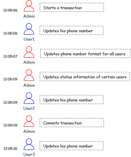
How it executes, in order:

• User 1 updates his phone number
• User 2 updates his phone number
• Admin updates phone number formats for all users
• Admin updates the status information of certain users
• User 3 updates his phone number

Queries in a transaction either all execute or all fail

When a transaction is to fail, each of its operations can be rolled back - meaning: for each operation, the reverse operation will be executed - and the database is brought back to the state it was at before beginning the transaction.

Note: the specific set of the query language that allows for transaction manipulation is called transaction control language - TCL

Data Integrity

DBMS will ensure Data Integrity through:

• Controlling that the data types are well respected
• Ensuring the atomicity of operations
• Allowing for the implementation of validation constraints on data Each DBMS will use an internal mechanism to keep a log of successfully executed operations an a log of faulty operations

Security and access control

This also an important feature of DBMS: DBMS allows to setup roles and give access to roles or users to objects in the database. This is done via a mechanism based on privileges. Privileges are a set of actions that a user or role an perform (ex. retrieving data, inserting new data, updating data, deleting data data, altering the structure of a table, a database, executing a function) and privileges are given on database objects: a database, a table, a column, views, procedures

Note: the specific set of query language that allows managing privileges is called Data Control Language - DCL

Backup and recovery

Backups are essential because errors tend to happen. It is necessary to be able to save the state of a Database and be able to get back to that state when needed. A DBMS will necessarily offer tools to perform backups an then restore those backups when needed.

Indexing

Indexing allows for fast retrieval of information. It improves performance by creating direct references to data sotred and avoiding going through the whole physical store to look for information. Depending on the DBMS, a different type of indexing can be used. the most popular one is B-tree, a concept a bit similar to a binary search tree, that allows for searches, access, insertions and deletions in a logarithmic time (meaninig the time to perform such operations grows slowly in comparison to the growth in the volume of data)

Fault Tolerance and High Volumetry

Professional DBMS will implement mechanisms for handling high volumes of data in a fault tolerant way. They will make it possible for a database to sit on multiple servers through replication using methods like the master-slave approach or clustering. They will also offer mechanisms like partioning or sharding and pagination to allow for storage and retrieval little chunks of data at the time for better performance

---

Intermediate SQL

Aggregate functions

• SUM(): adds together all values in a particular column
• MIN(): fetches the lowest value in a particular column
• MAX(): fetches the highest value in a particular column
• AVG(): calculates the average of a group of selected values
• COUNT(): counts how many rows are in a particular column

Group By

Simply put, group by separates data into groups that can be aggregated independently.

SELECT
	category,
	SUM(spend)
FROM product_spend
GROUP BY category;

we can group by multiple columns, whenever the aggregation we want depends on a combination of multiple attributes, not just one. Basically, you’re creating groups that are unique across all the columns in the GROUP BY clause.

rules to uphold when grouping by a column or more:

• every column in select that isn't inside an aggregate function must be in group by
• include a column in group by if you want to see results split by that column
• columns inside an aggregate function do not need to be in group by
• if we want to column in the result but not in group by, it must be aggregated somehow

Having

Due to WHERE's shortcomings in dealing with aggregated groups (mainly cuz it's for filtering rows before aggregation), HAVING comes in to filter groups after aggregation. Having lets us keep or discard entire groups based on a condition that usually involves aggregate functions like SUM(), COUNT(), AVG(),...

SELECT ticker, AVG(open)
FROM stock_prices
GROUP BY ticker
HAVING AVG(open) > 200;

	WHERE	HAVING
When it filters	Values BEFORE Grouping	Values after Grouping
Operates on data from	Individual rows	Aggregated values from groups of rows
example	SELECT username, followers FROM instagram_data WHERE followers > 1000;	SELECT country FROM instagram_data GROUP BY country HAVING AVG(followers) > 100;

HAVING can also be used with multiple conditions, we can add AND and whatever conditions necessary

Distinct

Used in conjunction with SELECT to return only distinct values

SELECT DISTINCT manufacturer FROM pharmacy_sales;

Arithmetic

We can use math expressions to transform column values

SELECT particle_speed / 10.0 + speed_offset
FROM particle_sensor_data WHERE (particle_position ^ 2) * 10.0 > 500 AND sensor_type = 'photon' AND measurement_day %  7 = 0;

Operator	Description	Example	Result
+	Addition	15 + 5	20
-	Subtraction	15 - 5	10
*	Multiplication	15 * 5	75
/	Division	15 / 5	3
%	Modulus (Remainder of Division)	14 % 5	4
^	Exponentiation (Not standard in all DBMS)	15 ^ 2	225
- (as a prefix)	Negation	-15	-15
for order of operations, sql follows PEMDAS

SQL Statement	Result	Explanation
SELECT 3 + 7 * 2;	17	Multiplication comes before addition.
SELECT (3 + 7) * 2;	20	Parentheses means addition happens first.
SELECT 10 / 2 + 3 * 4;	17	10/2 = 5, 3*4=12, so 5 + 12 = 17.
SELECT (10 / 2) + (3 * 4);	17	Same as above, but more explicit with parens!

Math

ABS(): Calculating absolute differences

SELECT    date,    ticker,   (close-open) AS difference,   ABS(close-open) AS abs_difference FROM stock_prices WHERE EXTRACT(YEAR FROM date) = 2023   AND ticker = 'GOOG';

ROUND(): Rounding numbers

SELECT    ticker,   AVG(close) AS avg_close,   ROUND(AVG(close), 2) AS rounded_avg_close FROM stock_prices WHERE EXTRACT(YEAR FROM date) = 2022 GROUP BY ticker;

CEIL() and FLOOR(): Rounding up and down

SELECT    date,   ticker,   high,   CEIL(high) AS resistance_level,   low,   FLOOR(low) AS support_level FROM stock_prices WHERE ticker = 'META' ORDER BY date;

POWER(): Calculating squared values

SELECT    date,   ticker,   close,   ROUND(POWER(close, 2),2) AS squared_close FROM stock_prices WHERE ticker IN ('AAPL', 'GOOG', 'MSFT') ORDER BY date;

MOD() or %: Modulus

SELECT    ticker,   close,   MOD(close, 5) AS price_remainder_mod,   close%5 AS price_remainder_modulo FROM stock_prices WHERE ticker = 'GOOG';

Division

In SQL, integer division discards the remainder from the output, providing only the integer part of the result, but we can use a couple of tricks to retain the decimal part:

CAST()

Convert one or both operands into decimal or floating-point data types

SELECT
  CAST(10 AS DECIMAL)/4,
  CAST(10 AS FLOAT)/4,
  10/CAST(6 AS DECIMAL),
  10/CAST(6 AS FLOAT);

Multiply by 1.0

Doing this converts an integer into a decimal or floating-point data type, allowing for the inclusion of decimal places in the result.

SELECT    10/6,   10*1.0/6,   10/6*1.0,   10/(6*1.0);

::DECIMAL/::FLOAT

The :: notation is a versatile tool to cast data types explicitly. When used for division, it signifies that you want the division to be executed with the specified data type, effectively achieving decimal or floating-point output.

SELECT    10::DECIMAL/4,   10::FLOAT/4,   10/4::DECIMAL,   10/4::FLOAT,   10::DECIMAL/6,   10::FLOAT/6;

NULL

Indicates the absence of a value, NULL doesn't represent a specific value but rather a missing or unknown piece of information

• IS NULL and IS NOT NULL: Used to identify null and non-null values.
• COALESCE(): Returns the first non-null value from a list of arguments.
• IFNULL(): Substitutes null value with a specified value specified.

Identifying null values with IS NULL and IS NOT NULL

SELECT * FROM goodreads WHERE book_title = NULL;

Takes multiple inputs and returns the first non-null value

SELECT COALESCE(book_rating, 0)
FROM goodreads;

Fill the gaps using IFNULL() with default values

SELECT    book_title,    IFNULL(book_rating, 0) AS rated_books FROM goodreads;

While both the COALESCE() and IFNULL() functions serve a similar purpose of handling NULL values, there is a key difference between them. COALESCE() function: Versatile for multiple arguments, it returns the first non-null value among them.

COALESCE(arg1, arg2, arg3, ...)

IFNULL() function: Handles two arguments, returning the second if the first is null; else, it returns the first.

IFNULL(expression, value_if_null)

CASE

Allows us to shape, transform, manipulate and filter data based on specified conditions

CASE in SELECT creates new columns, categorizes data or performs calculations based on specific conditions

SELECT
  column_1,
  column_2,
  CASE
    WHEN condition_1 THEN result_1
    WHEN condition_2 THEN result_2
    WHEN ... THEN ...
    ELSE result_3 -- If condition_1 and condition_2 are not met, return result_3 in ELSE clause
  END AS column_3_name -- Give your new column an alias
FROM table_1;

CASE in WHERE filters rows based on specific conditions

SELECT   column_1,   column_2
FROM table_1
WHERE CASE
		WHEN condition_1 THEN result_1
		WHEN condition_2 THEN result_2
		WHEN ... THEN ...
		ELSE result_3 -- If condition_1 and condition_2 are not met, return result_3 in ELSE clause   END;

JOIN

There are 4 types of joins:

• Inner join: only matches
• Left join: everything from left, plus matches
• Right join: everything from right, plus matches
• Full outer join: everything from both, matched if possible
• Cross join: every possible combination

INNER JOIN

• returns only the rows where there's a match in both tables
• if a row in one table has no corresponding match in the other, it will not appear in the result

SELECT c.customer_id, c.name, o.order_id
FROM customers c
INNER JOIN orders o
    ON c.customer_id = o.customer_id;

LEFT JOIN

• returns all rows from the left table, and the matched rows from the right table
• if there's no match on the right side, you'll still see the left row, with null values for the right side

SELECT c.customer_id, c.name, o.order_id
FROM customers c
LEFT JOIN orders o
    ON c.customer_id = o.customer_id;

RIGHT JOIN

• The opposite of left join
• returns all rows from the right table, matched rows from the left table
• if there's no match, the left side will show null

SELECT c.customer_id, c.name, o.order_id
FROM customers c
RIGHT JOIN orders o
    ON c.customer_id = o.customer_id;

FULL OUTER JOIN

• returns all rows from both tables
• rows that don't have a match on either side will still appear, with null for the missing columns

SELECT c.customer_id, c.name, o.order_id
FROM customers c
FULL OUTER JOIN orders o
    ON c.customer_id = o.customer_id;

CROSS JOIN

• returns the cartesian product of the two tables
• every row in table A is combined with every row in table B
• Typically used for generating combinations or when you deliberately want all pairings

SELECT from e.employee_name, p.project_name
FROM employees e
CROSS JOIN projects p;

DATETIME

Function	PostgreSQL	MySQL	SQL Server
Current Date	CURRENT_DATE	CURDATE()	CAST(GETDATE() AS DATE)
Current Time	CURRENT_TIME	CURTIME()	CAST(GETDATE() AS TIME)
Current DateTime	NOW()	NOW()	GETDATE()
UTC DateTime	CURRENT_TIMESTAMP	UTC_TIMESTAMP()	GETUTCDATE()
Extracting Parts of Date

Part	PostgreSQL	MySQL	SQL Server
Year	EXTRACT(YEAR FROM ts)	YEAR(ts)	YEAR(ts)
Month	EXTRACT(MONTH FROM ts)	MONTH(ts)	MONTH(ts)
Day	EXTRACT(DAY FROM ts)	DAY(ts)	DAY(ts)
Hour	EXTRACT(HOUR FROM ts)	HOUR(ts)	DATEPART(HOUR, ts)
Minute	EXTRACT(MINUTE FROM ts)	MINUTE(ts)	DATEPART(MINUTE, ts)
Second	EXTRACT(SECOND FROM ts)	SECOND(ts)	DATEPART(SECOND, ts)
Date Arithmetic

Operation	PostgreSQL	MySQL	SQL Server
Add Days	ts + INTERVAL '5 days'	DATE_ADD(ts, INTERVAL 5 DAY)	DATEADD(DAY, 5, ts)
Subtract Days	ts - INTERVAL '5 days'	DATE_SUB(ts, INTERVAL 5 DAY)	DATEADD(DAY, -5, ts)
Difference in Days	AGE(ts1, ts2) or ts1 - ts2	DATEDIFF(ts1, ts2)	DATEDIFF(DAY, ts1, ts2)

Formatting Dates

Task	PostgreSQL	MySQL	SQL Server
Format Date	TO_CHAR(ts, 'YYYY-MM-DD')	DATE_FORMAT(ts, '%Y-%m-%d')	FORMAT(ts, 'yyyy-MM-dd')
Parse String → Date	TO_DATE('2025-09-25', 'YYYY-MM-DD')	STR_TO_DATE('2025-09-25', '%Y-%m-%d')	CAST('2025-09-25' AS DATE)

Advanced SQL

CTEs

Common Table Expression create temporary tables to store results, making complex queries more readable and maintainable, these temp tables exist only for the duration of the main query, streamlining your analysis process

Subqueries

also known as inner queries, it's basically a query embedded within another, by nesting the queries we can generate tables to perform calculations and filter data within the main query. subqueries enable granular control over data, enhancing the precision of our analysis

---

pgAdmin 4 GUI Exploration

pgAdmin 4 is the graphical user interface (GUI) client for PostgreSQL. It provides a convenient way to interact with your databases, run queries, manage objects, and monitor database health. This guide offers a structured exploration of the main features and components of the pgAdmin 4 interface.

🗂️ Main Layout Overview

• Browser Panel (Left Sidebar)

  • Displays server groups, servers, databases, and objects in a tree structure.
  • Right-click on any node to create, view, or delete objects.

• Dashboard Panel (Main Workspace)

  • Displays monitoring widgets: sessions, locks, activity, etc.
  • Useful for server and database-level analytics.

• Toolbar (Top Bar)

  • Common actions like Create, Save, Run Query, Refresh, etc.
  • Allows access to Preferences, File operations, and Help menu.

🔑 Server & Connection Management

1. Registering a Server

   • Right-click “Servers” → “Register” → “Server”.
   • Provide connection details:
     • General Tab: Name, group.
     • Connection Tab: Host, port, username, password, maintenance DB.

2. Connecting to Server

   • Expand the server tree.
   • Prompted for password (if not saved).

3. Disconnection & Removal

   • Right-click server → Disconnect or Delete.

🧱 Database Object Navigation

• Databases
  • View schemas, tables, functions, sequences, and more.
• Schemas
  • Default public schema.
  • Logical grouping of tables and other objects.
• Tables
  • Explore columns, constraints, indexes, triggers, and data.

🧪 Query Tool

• Open by right-clicking a database or table → Query Tool.
• Features:
  • SQL editor with syntax highlighting and autocompletion.
  • Results grid for SELECT statements.
  • Execution plan visualizer.
  • Message tab with error/info logs.
• Shortcuts:
  • F5: Execute query
  • Ctrl+R: Clear output panel

📈 Dashboard & Monitoring

• Real-time charts:
  • CPU Usage
  • Active Sessions
  • TPS (Transactions per second)
• Object Statistics:
  • Table size
  • Tuple counts
  • Index usage
• Session Viewer:
  • Monitor current sessions and cancel queries.

🧰 Tools & Utilities

• Backup & Restore
  • Right-click DB or table → Tools → Backup/Restore
  • Configure format, location, and options.
• Maintenance
  • VACUUM, ANALYZE, REINDEX from GUI.
• ERD Tool (if enabled)
  • Visualize and manage table relationships.

⚙️ Preferences & Customization

• Navigate to: File → Preferences
  • Themes: Light/Dark
  • SQL Editor: Font, tab size, autocomplete behavior
  • Browser Tree: Node grouping and refresh policies

🛠️ Troubleshooting Tips

• Slow Interface?
  • Disable unnecessary dashboard widgets.
  • Increase query timeout settings.
• Connection Errors?
  • Check PostgreSQL server is running.
  • Verify credentials and network accessibility.

📚 Summary

Component	Function
Browser Tree	Navigation and object management
Query Tool	Writing and executing SQL queries
Dashboard	Real-time stats and monitoring
Tools	Backup, restore, maintenance
Preferences	Interface customization

✅ Recommended Usage Flow

1. Connect to PostgreSQL server.
2. Browse and explore schema objects.
3. Use Query Tool to run queries.
4. Monitor performance via Dashboard.
5. Backup or maintain databases as needed.

Version: pgAdmin 4 Compatibility: PostgreSQL 9.6+

---

Analyses